Integrate a mosaic tonsil dataset
In this notebook, we used SpaMosaic to integrate a mosaic tonsillar dataset that was measured by 10x Genomics Visium RNA and protein co-profiling technology. It has three sections where the first section consists of RNA and protein profiles while the second only has RNA expression and the third only has protein expression.
Data used in this notebook can be downloaded from google drive.
[1]:
import os
import scanpy as sc
from os.path import join

from spamosaic.framework import SpaMosaic

os.environ['CUBLAS_WORKSPACE_CONFIG'] = ':4096:8'  # for CuBLAS operation and you have CUDA >= 10.2
import spamosaic.utils as utls
from spamosaic.preprocessing import RNA_preprocess, ADT_preprocess, Epigenome_preprocess
[2]:
ad1_rna = sc.read_h5ad('./s1_adata_rna.h5ad')
ad1_adt = sc.read_h5ad('./s1_adata_adt.h5ad')
ad2_rna = sc.read_h5ad('./s2_adata_rna.h5ad')
ad3_adt = sc.read_h5ad('./s3_adata_adt.h5ad')
preprocessing
SpaMosaic expects batch-corrected low-dimensional representations for each modality as input. Therefore, for the raw count assays of each modality, SpaMosaic performs feature selection and dimension reduction to obtain the low-dimensional representations. Then, Harmony is performed to integrate these representations in each modality (optional, depending on the presence of strong batch effects).
In mosaic integration, SpaMosaic requires the input dataset in the following format:
{
    'rna':      [adata1_rna, adata2_rna,   None,         adata4_rna, ...],
    'protein':  [adata1_adt, None,         adata3_adt,   None,       ...],
    'atac':     [None,       adata2_atac,  None,         None,       ...],
    'histone':  [None,       None      ,   adata3_hist,  None,       ...],
    ...
}
In the dictionary, each key represents a modality and each modality key corresponds to list of anndata objects. Each anndata object contains modality-specific information for a particular section. For example, the first object adata1_rna under the ‘rna’ key holds the RNA profiles for the first section, while the first object adata1_adt under the ‘protein’ key holds protein profiles for the same section. If a section is not measured for a particular modality, its value in the list
is None. For instance, the first element under the ‘atac’ and ‘histone’ keys is None, indicating that the first section was not measured with ATAC or histone modality. All lists have the same length, which corresponds to the number of sections in the target dataset.
SpaMosaic employs contrastive learning to capture the relationships between modalities. To achieve this, it requires the modalities in a mosaic dataset to be directly or indirectly connected through one or multiple sections. If a pair of modalities occur in the same section, there is a direct connection between this pair of modalities, while an indirect connection requires multiple intermediary direct connections.
[4]:
input_dict = {
    'rna': [ad1_rna, ad2_rna, None],
    'adt': [ad1_adt, None,    ad3_adt]
}

input_key = 'dimred_bc'
Parameters in the following RNA_preprocess and ADT_preprocess function:
batch_corr: whether to perform batch correction with Harmonyfavor: following the standard ‘scanpy’ preprocessing workflow or an ‘adapted’ workflown_hvg: how many highly variable genes to selectbatch_key: the key in the row metadata that holds the batch labelskey: the key in.obsmthat will hold the output low-dimensional representations
After preprocessing, the low-dimensional representations can be accessed by: ad1_rna.obsm[input_key], ad2_rna.obsm[input_key], ad1_adt.obsm[input_key]…
[5]:
RNA_preprocess(input_dict['rna'], batch_corr=True, favor='scanpy', n_hvg=5000, batch_key='src', key=input_key)
ADT_preprocess(input_dict['adt'], batch_corr=True, batch_key='src', key=input_key)
Use GPU mode.
        Initialization is completed.
        Completed 1 / 10 iteration(s).
        Completed 2 / 10 iteration(s).
        Completed 3 / 10 iteration(s).
Reach convergence after 3 iteration(s).
Use GPU mode.
        Initialization is completed.
        Completed 1 / 10 iteration(s).
        Completed 2 / 10 iteration(s).
        Completed 3 / 10 iteration(s).
Reach convergence after 3 iteration(s).
training
SpaMosaic employs modality-specific graph neural networks to embed each modality’s input into latent space. In horizontal integration, all sections have only one modality, thus each section has only one set of embeddings.
The crucial parameters include:
intra_knns: how many nearest neighbors to consider when searching for spatial neighbors within each section (list or integer)inter_knn_base: how many nearest neighbors to consider when searching for mutual nearest neighbors between sections (integer)w_g: the weight for spatial-adjacency graph
The following parameters are recommended to use in complex integration scenarios, like varying resolution or size across sections
smooth_input: whethere to smooth the input representations (bool)smooth_L: number of LGCN layers for smoothing inputinter_auto_knn: whether to automatically balance the kNN during MNN searching (bool)rmv_outlier: whether to remove outlier of MNN (bool)contamination: percentage of removed MNN outlier
for training:
net: which graph neural network to use (only support wlgcn now)lr: learning raten_epochs: number of training epochsw_rec_g: the loss weight for reconstructing original graph structure. If the target dataset contains protein modality, we recommend a low value for w_rec_g (e.g., 0); if it contains epigenome modality, we recommend a high value for w_rec_g (e.g., 1).
[6]:
model = SpaMosaic(
    modBatch_dict=input_dict, input_key=input_key,
    batch_key='src', intra_knns=10, inter_knn_base=10, w_g=0.8,
    seed=1234,
    device='cuda:0'
)

model.train(net='wlgcn', lr=0.01, T=0.01, n_epochs=100)
batch0: ['rna', 'adt']
batch1: ['rna']
batch2: ['adt']
------Calculating spatial graph...
The graph contains 43260 edges, 4326 cells.
10.0000 neighbors per cell on average.
------Calculating spatial graph...
The graph contains 45190 edges, 4519 cells.
10.0000 neighbors per cell on average.
------Calculating spatial graph...
The graph contains 43260 edges, 4326 cells.
10.0000 neighbors per cell on average.
------Calculating spatial graph...
The graph contains 45210 edges, 4521 cells.
10.0000 neighbors per cell on average.
Searching MNN within rna
Finding MNN between (s1, s2) using KNN (10, 10)
Number of mnn pairs for rna:14704
Searching MNN within adt
Finding MNN between (s1, s3) using KNN (10, 10)
Number of mnn pairs for adt:13787
100%|███████████████████████████████████████████████████████████████████████████████████| 100/100 [00:03<00:00, 29.94it/s]
inference
After training, SpaMosaic can infer the modality-specific embedding for each section. These embeddings will be directly saved in original anndata objects. For example, the RNA-specific embeddings can be accessed by ad1_rna.obsm['emb'], ad2_rna.obsm['emb'], the protein-specific embeddings can be accessed by ad1_adt.obsm['emb'], ad3_adt.obsm['emb'].
The following infer_emb function will return a new list of anndata objects, which save the final/merged embeddings for spatial clustering. The final embeddings can be accessed by ad_embs[0].obsm['merged_emb'], ad_embs[1].obsm['merged_emb'], …
In mosaic integration, the final merged embeddings are obtained by averaging the modality-specific embeddings.
[7]:
ad_embs = model.infer_emb(input_dict, emb_key='emb', final_latent_key='merged_emb')
ad_mosaic = sc.concat(ad_embs)
ad_mosaic = utls.get_umap(ad_mosaic, use_reps=['merged_emb'])
/home/yanxh/anaconda3/envs/spamosaic-env/lib/python3.8/site-packages/tqdm/auto.py:21: TqdmWarning: IProgress not found. Please update jupyter and ipywidgets. See https://ipywidgets.readthedocs.io/en/stable/user_install.html
  from .autonotebook import tqdm as notebook_tqdm
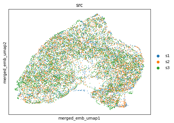
Visualize the final embeddings using UMAP plots, spot are colored by batch labels
[8]:
utls.plot_basis(ad_mosaic, basis='merged_emb_umap', color=['src'])
clustering
Parameters for the following utls.clustering function:
n_cluster: expected number of clustersused_obsm: the target key in thead_mosaic.obsmthat holds the embeddings for clustering inputalgo: which clustering algorithm to use,mclustorkmeans. Sometimesmclustcan fail to output clustering, it will automatically output thekmeansoutputs.key: the key in the row metadata that will hold the output clustering labels.
Generally, SpaMosaic works better with the mclust algorithm in spatial domain identification task. The final/merged embeddings are used as input for mclust and the clustering labels can be accessed by ad_mosaic.obs['mclust'].
[9]:
utls.clustering(ad_mosaic, n_cluster=6, used_obsm='merged_emb', algo='mclust', key='mclust')
utls.split_adata_ob(ad_embs, ad_mosaic, 'obs', 'mclust')
R[write to console]:                    __           __
   ____ ___  _____/ /_  _______/ /_
  / __ `__ \/ ___/ / / / / ___/ __/
 / / / / / / /__/ / /_/ (__  ) /_
/_/ /_/ /_/\___/_/\__,_/____/\__/   version 6.0.0
Type 'citation("mclust")' for citing this R package in publications.
fitting ...
  |======================================================================| 100%
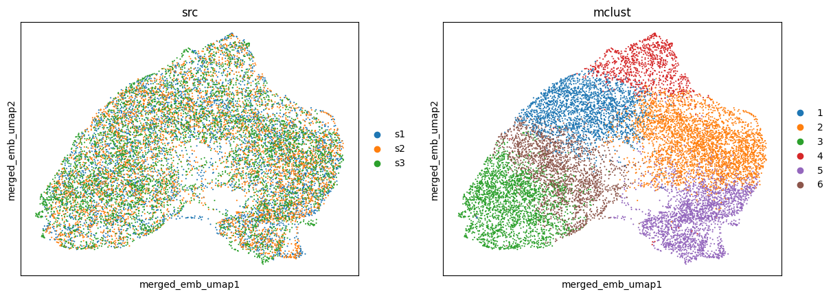
[10]:
utls.plot_basis(ad_mosaic, basis='merged_emb_umap', color=['src', 'mclust'])
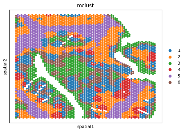
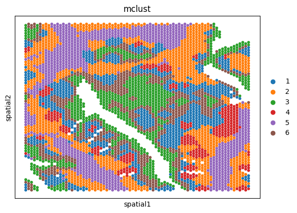
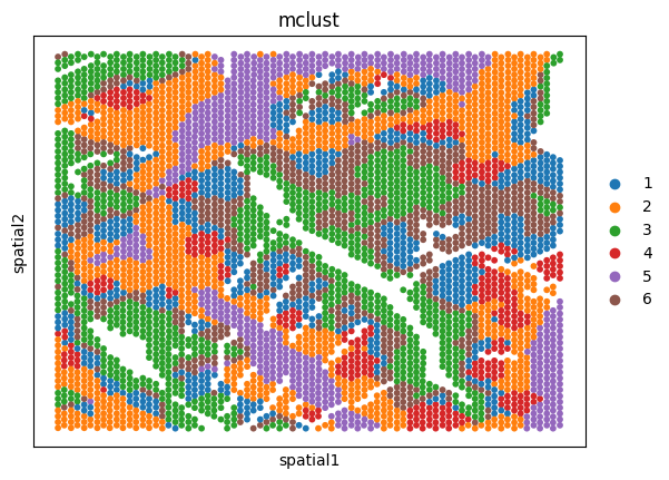
Spatial plots of clustering label for individual sections
[11]:
for ad in ad_embs:
    utls.plot_basis(ad, 'spatial', 'mclust', s=70)
[ ]: