Integrate three mouse brain sections in the RNA modality

In this notebook, we used SpaMosaic to integrate three postnatal mouse brain sections in the RNA modality. All three sections were measured by spatial-RNA-epigenome seq (Zhang et al., Nature. 2023). The first section consists of the transcriptome and ATAC profiles of a P21 mouse brain section in a capture area with 50×50 pixels, each 20 µm in diameter. The second section is a replicate experiment for the first section. It measured the spatial transcriptome and ATAC of a P21 mouse brain section with a capture array of 50×50 pixels, each 20 µm in diameter. The third section consists of the transcriptome and histone modification (H3K27ac) assays of a P21 mouse brain section with a capture array of 50×50 pixels, each 20 µm in diameter. We retained the transcriptome profiles of three sections for horizontal settings.

Data used in this notebook can be downloaded from google drive.

import os
import scanpy as sc
from os.path import join

import spamosaic
from spamosaic.framework import SpaMosaic

os.environ['CUBLAS_WORKSPACE_CONFIG'] = ':4096:8'  # for CuBLAS operation and you have CUDA >= 10.2

import spamosaic.utils as utls
from spamosaic.preprocessing import RNA_preprocess, ADT_preprocess, Epigenome_preprocess

ad1_rna = sc.read_h5ad('./s1_adata_rna.h5ad')
ad2_rna = sc.read_h5ad('./s2_adata_rna.h5ad')
ad3_rna = sc.read_h5ad('./s3_adata_rna.h5ad')

# change the batch label; `src` is the key in the row metadata that holds the batch labels
ad3_rna.obs['src'] = 's3'
# modify the barcode
ad3_rna.obs_names = [x.replace('s1-', 's3-') for x in ad3_rna.obs_names]

# intersection of features
shared_genes = ad1_rna.var_names.intersection(ad2_rna.var_names).intersection(ad3_rna.var_names)

preprocessing

SpaMosaic expects batch-corrected low-dimensional representations for each modality as input. Therefore, for the raw count assays of each modality, SpaMosaic performs feature selection and dimension reduction to obtain the low-dimensional representations. Then, Harmony is performed to integrate these representations in each modality (optional, depending on the presence of strong batch effects).

By default, the feature selection and dimension reduction consist of following steps:

• RNA assays: highly variable gene selection \(\rightarrow\) log normalization \(\rightarrow\) PCA

• epigenome assays: highly variable peak selection \(\rightarrow\) TF-IDF transformation \(\rightarrow\) log normalization \(\rightarrow\) PCA

• protein assays: centered log ratio normalization \(\rightarrow\) PCA

In horizontal integration, SpaMosaic requires the input in the format of

{
    'modality_name': [adata1, adata2, adata3, ...]
}

In the dictionary, each key represents a modality and each modality key corresponds to list of anndata objects. Each anndata object contains modality-specific information for a particular section.

input_dict = {
    'rna':  [ad1_rna[:, shared_genes].copy(),  ad2_rna[:, shared_genes].copy(), ad3_rna[:, shared_genes].copy()],
}

input_key = 'dimred_bc'

Parameters in the following RNA_preprocess function:

• batch_corr: whether to perform batch correction with Harmony

• n_hvg: how many highly variable genes to select

• batch_key: the key in the row metadata that holds the batch labels

• key: the key in .obsm that will hold the output low-dimensional representations

After preprocessing, the low-dimensional representations can be accessed by: ad1_rna.obsm[input_key], ad2_rna.obsm[input_key], …

RNA_preprocess(input_dict['rna'], batch_corr=True, n_hvg=5000, batch_key='src', key=input_key)

Use GPU mode.
        Initialization is completed.
        Completed 1 / 10 iteration(s).
        Completed 2 / 10 iteration(s).
        Completed 3 / 10 iteration(s).
Reach convergence after 3 iteration(s).

training

SpaMosaic employs modality-specific graph neural networks to embed each modality’s input into latent space. In horizontal integration, all sections have only one modality, thus each section has only one set of embeddings.

The crucial parameters include:

• intra_knns: how many nearest neighbors to consider when searching for spatial neighbors within each section (list or integer)

• inter_knn_base: how many nearest neighbors to consider when searching for mutual nearest neighbors between sections (integer)

• w_g: the weight for spatial-adjacency graph

The following parameters are recommended to use in complex integration scenarios, like varying resolution or size across sections

• smooth_input: whethere to smooth the input representations (bool)

• smooth_L: number of LGCN layers for smoothing input

• inter_auto_knn: whether to automatically balance the kNN during MNN searching (bool)

• rmv_outlier: whether to remove outlier of MNN (bool)

• contamination: percentage of removed MNN outlier

for training:

• net: which graph neural network to use (only support wlgcn now)

• lr: learning rate

• n_epochs: number of training epochs

• w_rec_g: the loss weight for reconstructing original graph structure. If the target dataset contains protein modality, we recommend a low value for w_rec_g (e.g., 0); if it contains epigenome modality, we recommend a high value for w_rec_g (e.g., 1).

model = SpaMosaic(
    modBatch_dict=input_dict, input_key=input_key,
    batch_key='src', intra_knns=10, inter_knn_base=10, w_g=0.8,
    seed=1234,
    device='cuda:0'
)

model.train(net='wlgcn', lr=0.001, n_epochs=60, w_rec_g=1.)

batch0: ['rna']
batch1: ['rna']
batch2: ['rna']
------Calculating spatial graph...
The graph contains 23720 edges, 2372 cells.
10.0000 neighbors per cell on average.
------Calculating spatial graph...
The graph contains 24970 edges, 2497 cells.
10.0000 neighbors per cell on average.
------Calculating spatial graph...
The graph contains 23860 edges, 2386 cells.
10.0000 neighbors per cell on average.
Searching MNN within rna
Finding MNN between (s1, s2) using KNN (10, 10)
Finding MNN between (s1, s3) using KNN (10, 10)
Finding MNN between (s2, s3) using KNN (10, 10)
Number of mnn pairs for rna:15914

100%|█████████████████████████████████████████████████████████████████████████████████████| 60/60 [00:04<00:00, 12.83it/s]

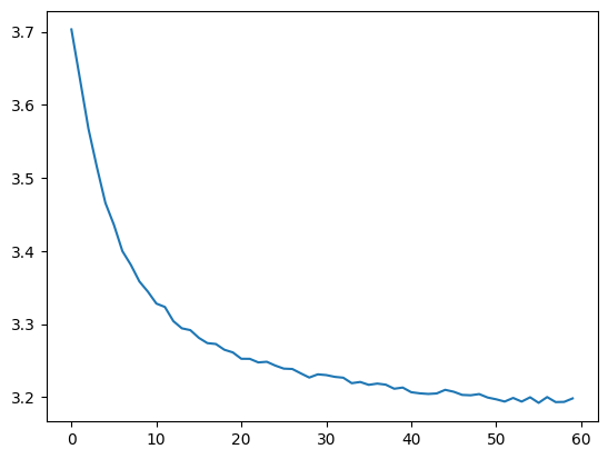
Tracking the loss history

import matplotlib.pyplot as plt
plt.plot(model.loss_rec)

[<matplotlib.lines.Line2D at 0x7f516c7541f0>]

inference

After training, SpaMosaic can infer the modality-specific embedding for each section. These embeddings will be directly saved in original anndata objects. For example, the RNA-specific embeddings can be accessed by ad1_rna.obsm['emb'], ad2_rna.obsm['emb'], ….

The following infer_emb function will return a new list of anndata objects, which save the final/merged embeddings for spatial clustering. The final embeddings can be accessed by ad_embs[0].obsm['merged_emb'], ad_embs[1].obsm['merged_emb'], …

Since we have only modality in horizontal integration, the final/merged embeddings are exactly the same as the RNA-specific embeddings.

ad_embs = model.infer_emb(input_dict, emb_key='emb', final_latent_key='merged_emb')
ad_mosaic = sc.concat(ad_embs)
ad_mosaic = utls.get_umap(ad_mosaic, use_reps=['merged_emb'])

/home/yanxh/anaconda3/envs/spamosaic-env/lib/python3.8/site-packages/tqdm/auto.py:21: TqdmWarning: IProgress not found. Please update jupyter and ipywidgets. See https://ipywidgets.readthedocs.io/en/stable/user_install.html
  from .autonotebook import tqdm as notebook_tqdm

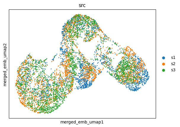
Visualize the final embeddings using UMAP plots, spot are colored by batch labels

utls.plot_basis(ad_mosaic, basis='merged_emb_umap', color=['src'])

clustering

Parameters for the following utls.clustering function:

• n_cluster: expected number of clusters

• used_obsm: the target key in the ad_mosaic.obsm that holds the embeddings for clustering input

• algo: which clustering algorithm to use, mclust or kmeans. Sometimes mclust can fail to output clustering, it will automatically output the kmeans outputs.

• key: the key in the row metadata that will hold the output clustering labels.

Generally, SpaMosaic works better with the mclust algorithm in spatial domain identification task. The final/merged embeddings are used as input for mclust and the clustering labels can be accessed by ad_mosaic.obs['mclust'].

utls.clustering(ad_mosaic, n_cluster=7, used_obsm='merged_emb', algo='mclust', key='mclust')
utls.split_adata_ob(ad_embs, ad_mosaic, 'obs', 'mclust')

R[write to console]:                    __           __
   ____ ___  _____/ /_  _______/ /_
  / __ `__ \/ ___/ / / / / ___/ __/
 / / / / / / /__/ / /_/ (__  ) /_
/_/ /_/ /_/\___/_/\__,_/____/\__/   version 6.0.0
Type 'citation("mclust")' for citing this R package in publications.

fitting ...
  |======================================================================| 100%

UMAP plots with batch label and mclust label

utls.plot_basis(ad_mosaic, basis='merged_emb_umap', color=['src', 'mclust'])

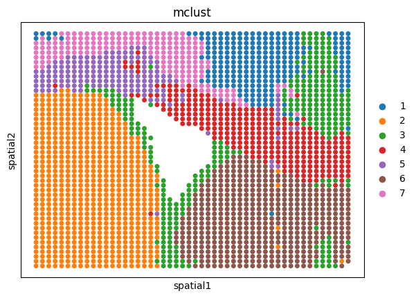
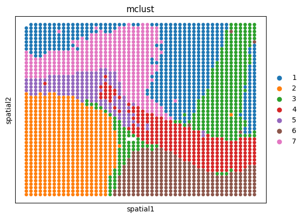
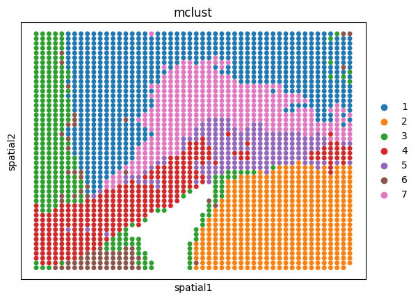
Spatial plots of clustering label for individual sections

sizes = [100, 100, 100]
for i, ad in enumerate(ad_embs):
    utls.plot_basis(ad, 'spatial', 'mclust', s=sizes[i])